
Data analytics is a major force in the current zeitgeist. Analytics are the eyes and ears on a very wide variety of domains (society, climate, health, etc.) to perform an even wider variety of tasks (such as understanding commercial trends, the spread of COVID-19, and finding exoplanets). In this article, I will discuss some fundamentals of data analytics and show how to get started with analytics in Python. Finally, I will show the whole process at work on a simple data analytics problem.
A Primer on Data Analytics
Data analytics uses tools from statistics and computer science (CS), such as artificial intelligence (AI) and machine learning (ML), to extract information from collected data. The collected data is usually very complex and voluminous, and it cannot be interpreted easily (or at all) by humans. Therefore, the data on its own is useless. Information lies hidden within the data, and it takes many forms: repeating patterns, trends, classifications, or even predictive models. You can use this data to uncover insights and build knowledge of the problem you are studying. For example, suppose you wish to measure the traffic in a parking lot that is monitored by a network of IoT sensors covering the whole city. Reading a single occupancy sensor doesn't say anything about the traffic on its own. Neither do the readings of all the parking sensors of the city without any more context. But the timestamped percentage of occupied places within the monitored parking lot does tell us something, and we use this information to derive insights, such as the times of day with maximum traffic.
Learning the mathematical background and analytics tools is only half the journey. Field expertise (experience on the problem that is being studied) is equally important. Some data scientists come from a statistics background, others are computer scientists who pick up the statistics as they go, and many are people starting from a field of expertise who need to learn both the statistics and the computing tools.
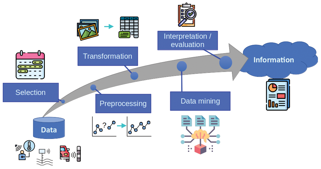
One important approach to data analytics is to use the Knowledge Discovery and Data Mining (KDD) model [1] – also known as Knowledge Discovery in Databases. The KDD process (see Figure 1) takes as input raw data from diverse sources (sensors, databases, logs, polls, etc.) and outputs information in the form of graphics, reports, and tables. The process has 5 steps:
- Selection – normally data sources are way more comprehensive than needed. Sensors might collect data from time periods or spatial locations that are out of the interest range or variables that are of no interest to the problem. This step narrows down the data that we know contains the information of interest. In the case of the parking example, we may only want to select data referring to the parking we want to monitor, as opposed to other parking spots throughout the city.
- Preprocessing – data is dirty; in other words, it may contain wrong or missing values caused by measurement errors or system failures. These errors can cause problems down the line, such as failures (in the best case) or hidden biases in the extracted information (in the worst case). Detecting wrong and missing data and filling it or dropping samples is part of the preprocessing stage. In the parking example, your might find null values when many parking sensors fail to send a reading or inconsistent values such as negative numbers.
- Transformation – once a clean dataset is in place, you might need to change its format to fit the requirements of the next stage. Tasks such as binning, converting from strings to numbers, obtaining parameters from images, etc. are just some of the thousands of possible actions in this stage. For the parking lot example, you might wish to do some binning, transforming the timestamp into a label representing an hour of a specific day.
- Data mining – this is the core of the whole KDD process. Data mining uses algorithms that extract the information from the clean, appropriately formatted data. Mining could consist of simple statistical computations (averages, standard deviations, and percentiles) or complex ML/AI processes (such as deep learning or unsupervised classification). In the parking lot example, I might wish to extract a time profile that represents the occupancy of the parking lot per hour. The process might be something like calculating the percent of occupied places per hour and day, and then averaging for several days at the same hour.
- Interpretation/evaluation – after you extract the necessary information, you still need one more step in which the results are validated before using the data to generate insights. Especially for complex outputs, such as predictive models, you need to evaluate the accuracy (normally with a separate validation dataset that was not used for the data mining process). Finally, you can use the information to generate insights or predictions. In the parking example, the resulting model could be used in a report that highlights the need for expanding the lot due to saturation at peak hours.
All of these tasks that form part of the KDD process must be supported by a computing platform. You'll need appropriate network connections to the sources, data storage, and a rich toolset to preprocess, transform, and mine the data. Linux is the ideal platform that provides all of these tools, thanks to its great network capabilities, the availability of databases (both small like SQLite and large, unstructured databases like MongoDB) and the great variety of FOSS tools for data processing and representation (such as LaTeX, gnuplot, or web servers for interactive and real-time reports). Among data scientists, Python stands out as an easy and capable programming language with a very comprehensive set of libraries for processing data from very diverse fields. And all of this comes with the advantages of FOSS.
| Updating with Pip |
|---|
It may seem redundant to have a package manager for Python when there are so many wonderful distro-specific package managers in Linux. But pip has some unique functionality that make it specially useful. Pip has a browsable repository, where the latest versions of libraries are promptly available. You can download and upgrade packages throughout the life cycle of a project, to integrate new functions or fixes. The first package you must upgrade is pip itself: pip install pip --upgrade. This should be done normally right after creating a new virtual environment. In general, to upgrade installed packages, enter pip install package --upgrade. |
The Python Programming Language
The principal benefits of Python are its ease of use, code clarity, and extensibility. Another important advantage of Python is the very wide ecosystem of libraries for many different fields. See the box entitled "Python Elements" for more on the basic components of the Python environment. No matter the topic (astronomy, macroeconomics, personal accounting, computer vision …), you will find a library in Python tailored to it. Coincidentally, data mining is also applicable to many different fields. The availability of both field-specific libraries and data analytics libraries makes Python quite appealing to data scientists. The box entitled "Python Data Science Libraries" highlights some of the important libraries used with data analytics applications.
| Python Data Science Libraries |
|---|
|
One supreme advantage of Python over other platforms is the rich ecosystem of libraries for data analytics, along with a myriad of smaller, field-specific libraries. Important libraries include:
|
| Python Elements |
|---|
|
The Python environment consists of several important elements, including the Python interpreter, the package manager, the shell, and the virtual environment manager. The interpreter is the virtual machine that reads and executes the code. A Python interpreter is usually present in most Linux distributions by default. Although most users rely on the vanilla interpreter (CPython), there are several alternative, specialized interpreters, such as Jython (integrated with the Java VM), PyPy (more performant than vanilla Python), or MicroPython (geared towards microcontrollers). Due to compatibility with libraries, vanilla Python is recommended for most of the tasks. The package manager downloads and installs libraries that can be used to extend the basic functionality of Python. The default package manager is called pip, and it has an online repository of more than 300,000 libraries called the Python Package Index (PyPI) [2]. An alternative to pip is Conda, which is related to the Anaconda Python Distribution. Anaconda packages the basic data science tools of Python, and it is especially useful for Windows and macOS users, where Python is not that well integrated into the system. Anaconda is also available for Linux, but it may add one layer of complexity in exchange of providing a sane collection of preinstalled packages. See Table 1 for a comparison between Anaconda Python and vanilla Python in Linux. Both Conda and pip can coexist in an install, but it is better to not mix them up if possible. Some package developers also distribute their libraries without integrating them into any repository. In that case, there are several common installation methods ( Another important element is the shell, which is the interactive interface to the interpreter, not unlike a terminal like Bash or Zsh. The basic shell is offered by the interactive mode of the vanilla Python interpreter. It can be invoked by calling python in a terminal (see Figure 2), and it can be used for small tasks and testing out simple code. IPython offers an improved interactive experience, with functions such as syntax highlighting and code completion. You can also use IDEs, such as PyCharm (which has a FOSS community edition) or Spyder (which will be familiar to users coming from MATLAB). A final important component is the virtual environment manager, which is a utility that creates isolated setups of the Python interpreter and packages for different projects. There is a base environment, associated with the system Python interpreter that is rooted within the basic OS filesystem. The virtual environments inherit the packages from the base environment and are rooted in a specific directory (normally within the home directory of the user). All the previously described elements can "live" either in the base environment or within a virtual environment. The basic manager included with Python is venv. While there are many other compatible alternatives (mainly to support older versions of Python), it is good practice to use venv. Another alternative available to Anaconda users is Conda, which also has the capability of creating virtual environments. Conda cannot be mixed with 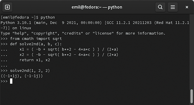
|
| Anaconda | Vanilla Python |
|---|---|
| Pro: All data science packages in one package. | Con: Need to install packages one by one. |
| Pro: Includes Anaconda Navigator, a GUI for managing the environment. | Con: Need to manually manage everything (not a con for many people). |
| Con: Uses the Conda package manager, which is not as complete as pip and interferes with it. | Pro: Has fewer "moving parts." |
| Con: Anaconda is not that well integrated into Linux package managers. | Pro: Python is very well integrated into most Linux distributions, unlike in Windows or macOS. |
Most Linux variants already have Python installed by default, or as a dependency of another package. But normally, only the interpreter is installed by default, so you need to manually install the rest of the elements. Table 2 shows the names of the Python interpreter, the pip package manager, and the venv library for some of the most popular distributions. Note that in most distributions, you must explicitly indicate that you are installing Python 3, to avoid confusion with Python 2 (which was deprecated in 2020, but is still a dependency of some software packages). When calling the interpreter, you must make sure that Python 3 is invoked, not Python 2. For instance, in Ubuntu, Debian, and openSUSE, you need to explicitly use the python3 command when invoking the interpreter. You can fix this in Ubuntu and Debian by installing the package python-is-python3. Another way to fix this problem is to use a use a virtual environment, where the default interpreter of the system is overridden.
| Component | Ubuntu/Debian | Fedora | Arch | openSUSE |
|---|---|---|---|---|
| Basic environment | python3, python3-pip, python3-venv, python-is-python3 | python3, python3-pip | python, python-pip | python3, python3-pip |
| Jupyter | python3-jupyter (no JupyterLab) | python3-notebook (no JupyterLab) | jupyterlab | python3-jupyterlab |
| NumPy | python3-numpy | python3-numpy | python-numpy | python3-numpy |
| Pandas |
python3-pandas |
python3-pandas |
python-pandas |
python3-pandas |
| Scikit-learn | python3-sklearn |
python3-scikit-learn |
python-scikit-learn | python3-sklearn |
|
Matplotlib |
python3-matplotlib |
python3-matplotlib |
python-matplotlib | python3-matplotlib |
| Seaborn | python3-seaborn | python3-seaborn |
python-seaborn |
python3-seaborn |
| Keras | python3-keras | Not in default repositories | python-keras | python3-keras |
Once the basic packages are installed, you can proceed to create a virtual environment. Although this step is optional, it is highly recommended when working with many different projects in parallel, which is normal in the life of a data scientist. A virtual environment will have a root folder with its own Python interpreter and its own package selection. The new Python interpreter will have access to the packages of the system interpreter. Note that, if Python 2 and Python 3 coexist in the system, a virtual environment created with Python 3 will only have access to the packages of the Python 3 system interpreter. Any package you install in the virtual environment will only be accessible within it. Also, you do not need to call python3 or pip3 explicitly, because within the virtual environment, only Python 3 is available.
To create a new virtual environment, open a terminal, cd into the directory where you want to create it, and run the following command:
# python3 -m venv new_environment_root
where new_environment_root can be any name. This command will only create the environment; you will not be able to use it until you activate it. For that, run the following command without changing the directory:
# source new_environment_root/bin/activate
This command will modify the terminal session to use the virtual environment's interpreter, along with the packages it can access. It will also change the behavior of the pip package manager, so packages are installed in the virtual environment. If you install a package that is also installed in the system, it will be overriden only within the virtual environment. This is ideal for when you need a specific version of a package. When you are done working with the environment, change the terminal session back with:
# deactivate
Setting Up Jupyter
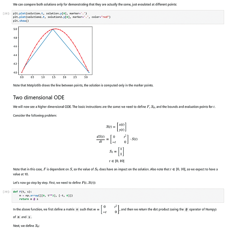
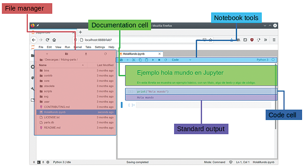
JupyterLab and Jupyter Notebooks are very important components in the Python data analytics environment. Jupyter proposes a completely different way of using Python, by providing an experimentation + coding + documentation workflow. In JupyterLab, you can create notebooks (Figure 3), which contain both code cells (that can be run in an interactive way and in no particular order) and documentation cells (which can contain Markdown, HTML, and LaTeX code). Because Jupyter lets you run different cells in a nonlinear fashion, it is a particularly useful environment for experimenting and doing exploratory data analytics. The output of code cells (both in the form of text or graphics) is also embedded in the document. We can therefore produce comprehensive documents with interactive code and even graphics, which we can use to document the process of data analytics.
Once you have Python installed in the system and a virtual environment to work in, you can start an interactive session with the interpreter or run scripts right away; but in order to use a powerful data science environment, you must install some tools and packages. The first one is JupyterLab. You have two installation options: using pip or using the OS package manager. Each method has its own advantages and disadvantages.
To install Jupyter with pip, run:
# pip install jupyterlab
This command will make JupyterLab available to the current virtual environment (if none is activated, it will install it on the system's Python installation) and will download the latest version. Once Jupyter is installed, you will have to upgrade manually from time to time (see the "Upgrading with Pip" box).
The other way of installing JupyterLab is using the OS package manager, which will make it available to all the virtual environments and will subject it to the update cycle of the OS, but will not install the latest version. Especially for distributions that use oldish packages (Debian Stable, Ubuntu LTS …), the installed version might be significantly outdated. Table 2 shows the name of the package for Jupyter in the main distributions.
Regardless of how you install it, to run JupyterLab, execute the following in a terminal while the virtual environment is active:
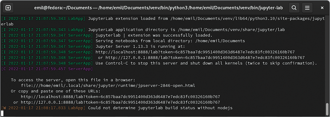
# jupyter-lab
This command will launch a server in port 8888 by default (Figure 4). The server shows a URL that can be opened in a browser to access the JupyterLab interface. The server will attempt to launch the default browser. Note that the server window must not be closed while working with Jupyter.
The web interface (Figure 5) will allow you to create new notebooks (which is the default document type for Jupyter) in the directory you select in the file manager. Figure 5 shows the JupyterLab screen, with the different areas marked. At the left side, you will find the file browser, where you can manage directories. On the right side is the main working area, where you will find a tabbed interface for the different notebooks. To create a new notebook, press the + button above the file explorer, which will open a new tab that offers the possibility of creating several new objects. Within the notebook, you will see documentation cells, where we can write Markdown, LaTeX, or HTML expressions, and code cells, where you write Python code. The code produces output right below the code cell, with text or graphic output.
Setting Up the Data Science Libraries
The final step is to install the main libraries. Again, just like with JupyterLab, you have the option of installing them with pip:
# pip install numpy pandas matplotlib sklearn
or with the OS package manager (Table 2).
This setup leaves you an environment that is ready both for exploratory data analytics, using JupyterLab, and for large batch processing, using the Python interpreter in script mode. Note that JupyterLab allows you to export a notebook to a Python script. You can also distribute results and documentation using Jupyter notebooks, to report data analytics work to clients. There is one more step that some users might want to take, depending on the specific data analytics project, and that is to install additional Python libraries. PyPI lists all the libraries available in pip. It is good practice to explore the package index before a big project and assess the available field-specific libraries, as well as their maturity and compliance with project requirements.
Example
Suppose I want to understand the behavior of the traffic in a parking lot. I will obtain a profile that shows the hourly average occupancy of the parking lot based on data collected in several measurement campaigns, at different days, in different points of the city. First, I need to retrieve the raw data. For this example, I will use the Birmingham Parking dataset, which was used in research work on Smart Cities [2]. Dowload the full dataset using wget:
wget https://archive.ics.uci.edu/ml/machine-learning-databases/00482/dataset.zip
You can enter this command in a terminal window, or you can use the special character ! within Jupyter to run a command in an embedded terminal. Next, unzip the data with unzip.
Given the great variety of formats, processes, and policies of data collection, dataset retrieval will look different each time; sometimes you need to download a ZIP file, sometimes you might just go to a database, or other times you might need to retrieve an SD card from an embedded system. That's the beauty of data science: Each project starts and develops in a different way.
For this example, I will include the Pandas data analytics library. Pandas completely changes the data workflow in Python, making it much more intuitive and easy. Internally, Pandas uses the mechanisms provided by NumPy, thus inheriting its efficiency. One common scenario is to load the data into a Pandas object, on which to perform preliminary data analysis tasks (especially the selection, preprocessing, and transformation stages).
The first step is to read the contents of the file into Pandas DataFrame, using the function read_csv() (Figure 6), to which you pass the mandatory filename parameter and an optional parse_dates parameter to force it to interpret one column as a date-time field. You can then visualize the contents loaded from the file with display().
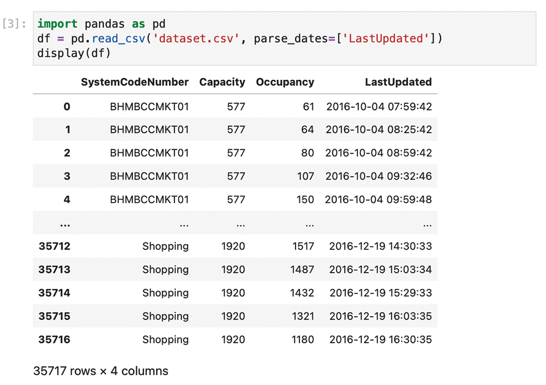
As you can see in Figure 6, the data appears in columns. The first column is SystemCodeNumber, which is an identifier of the parking lot. The second column (Capacity) shows the total capacity of the lot, and the third one (Occupancy) shows the current number of occupied parking spaces. Finally, LastUpdated shows the time and date of the last sensor reading.
The next step is to apply a selection process to only take the samples of the NIA North parking lot. For this step, use the .loc property of the Pandas DataFrame object, which allows you to filter the rows. The code shown in Figure 7 filters all the entries in df, where the parking lot name is 'NIA North'.

The .loc property is very powerful, allowing filtering with a great variety of conditions. More information can be found in the Pandas documentation.
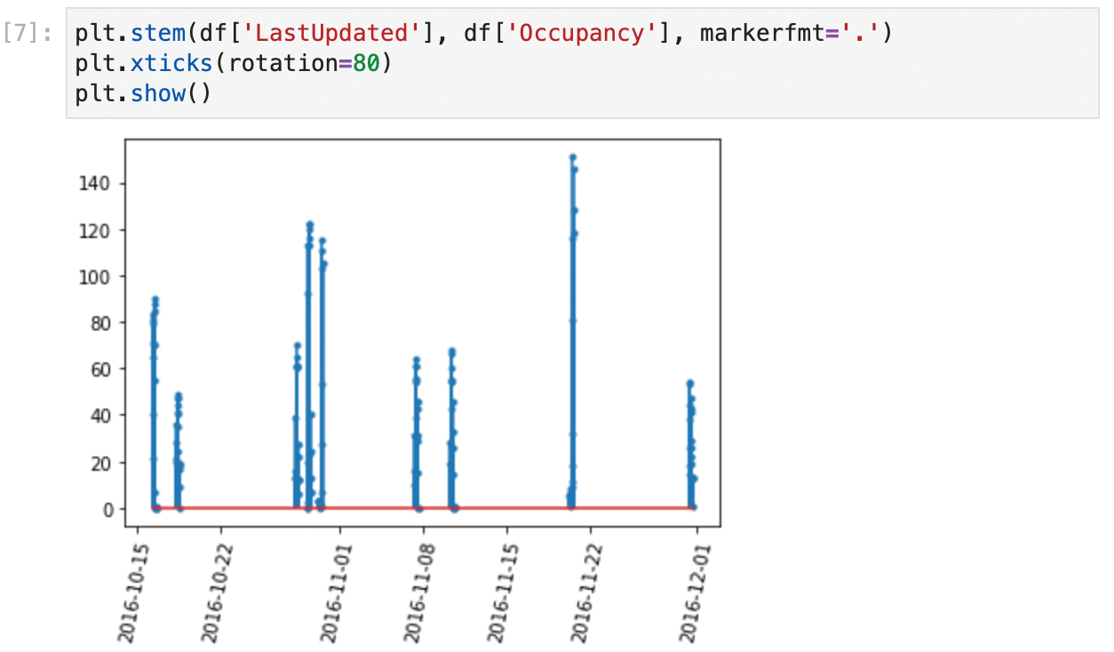
You now have the data of interest in df. Nevertheless, data in the real world normally comes with errors and/or outliers. This dataset is not an exception, as you can see in the Matplotlib plot shown in Figure 8.
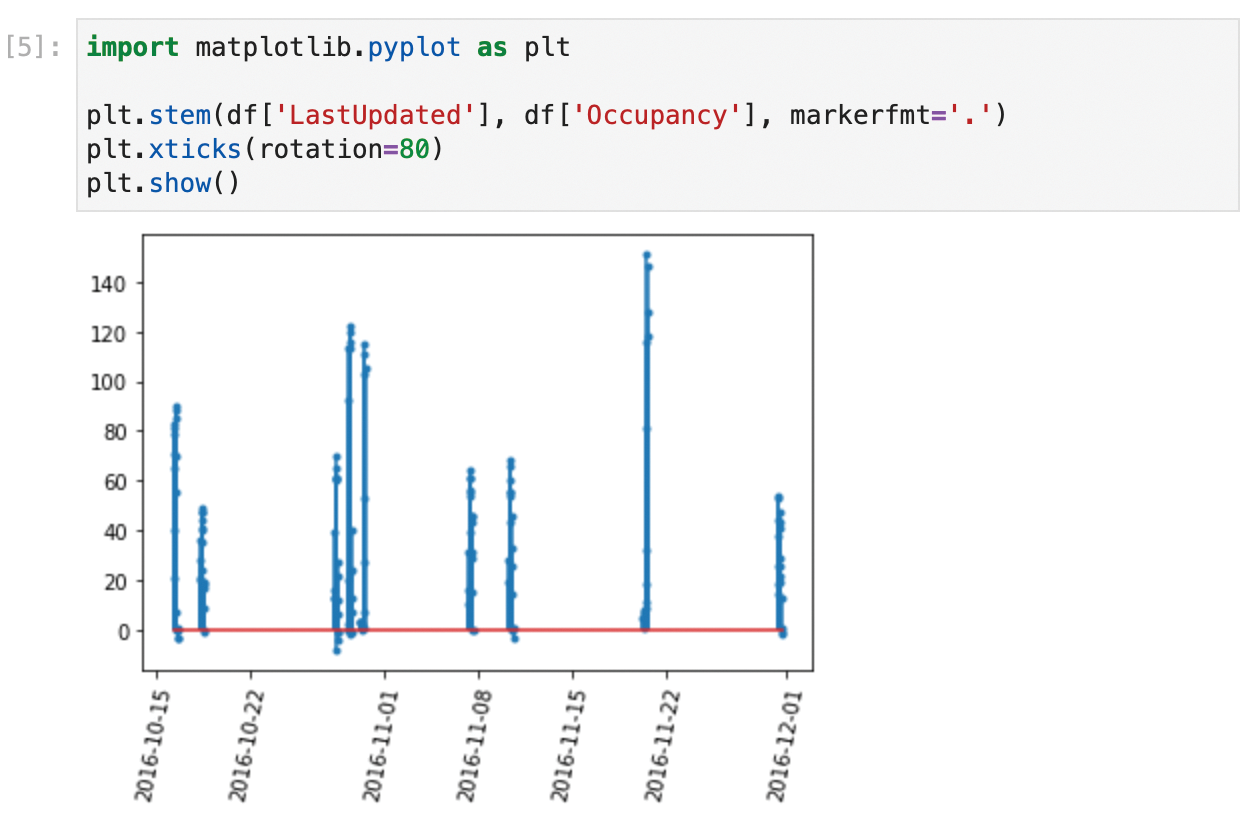
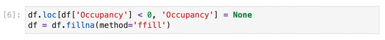
In Figure 8, the readings only come from isolated days where measurements were taken. Also, some values of occupancy are lower than 0 (which is impossible), so I need to remove these wrong values. These errors will be different in each project, so normally you will have to spend some time in this phase thinking of possible errors and chasing them. It takes some experience to do this quickly, and normally you might miss some errors and detect them further down the road. When you do so, you need to come back to this part of the study and add the appropriate mechanisms to detect them. Thanks to Jupyter's nonlinear workflow, you can do this easily by adding or editing cells in the appropriate places. Again, the .loc method will come in handy. In this case, I will replace the wrong values with None. If I knew a method to directly correct them, I could have used that method instead. Next, I will fill in the missing values with some generic value. Pandas offers the .fillna() method for filling missing data. You can fill in a constant value (for instance, ), or use the last known value. I will use the last known value in this case, because a good estimation for occupancy of a parking lot is the occupancy that it had previously. The code in Figure 9 shows the command for cleanup, and Figure 10 shows the corrected data.
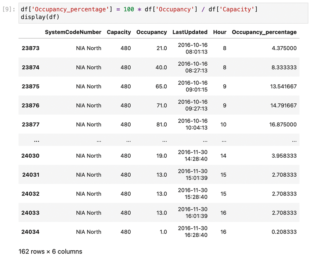
Next is the transformation step. Start by thinking about what the modeling process (the next step) requires. Because you want to do an hourly average of the occupancy expressed as a proportion, you'll need two transformations. First, you need to extract the hour from the date-time field, as shown in Figure 11. With this, you can create a new column that only contains the hour. Next, you need to compute a new column that expresses the occupancy as a proportion, instead of an absolute value (Figure 12). Figure 12 also shows the dataset with the new columns.

To build the model in the data mining step, you actually only need the last two columns. Start by taking all the samples for each hour, and then calculate the average of the occupancy. In other words, group by the Hour column and calculate the mean. Grouping is such a common task that Pandas offers the groupby shorthand (Figure 13).
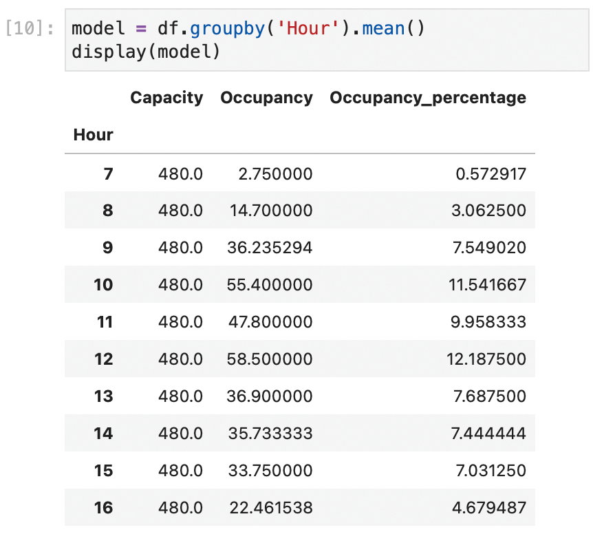
groupby will result in a new data frame, model, indexed with the unique values of Hour, and that new data frame contains the average value of all the other numerical fields grouped by Hour.
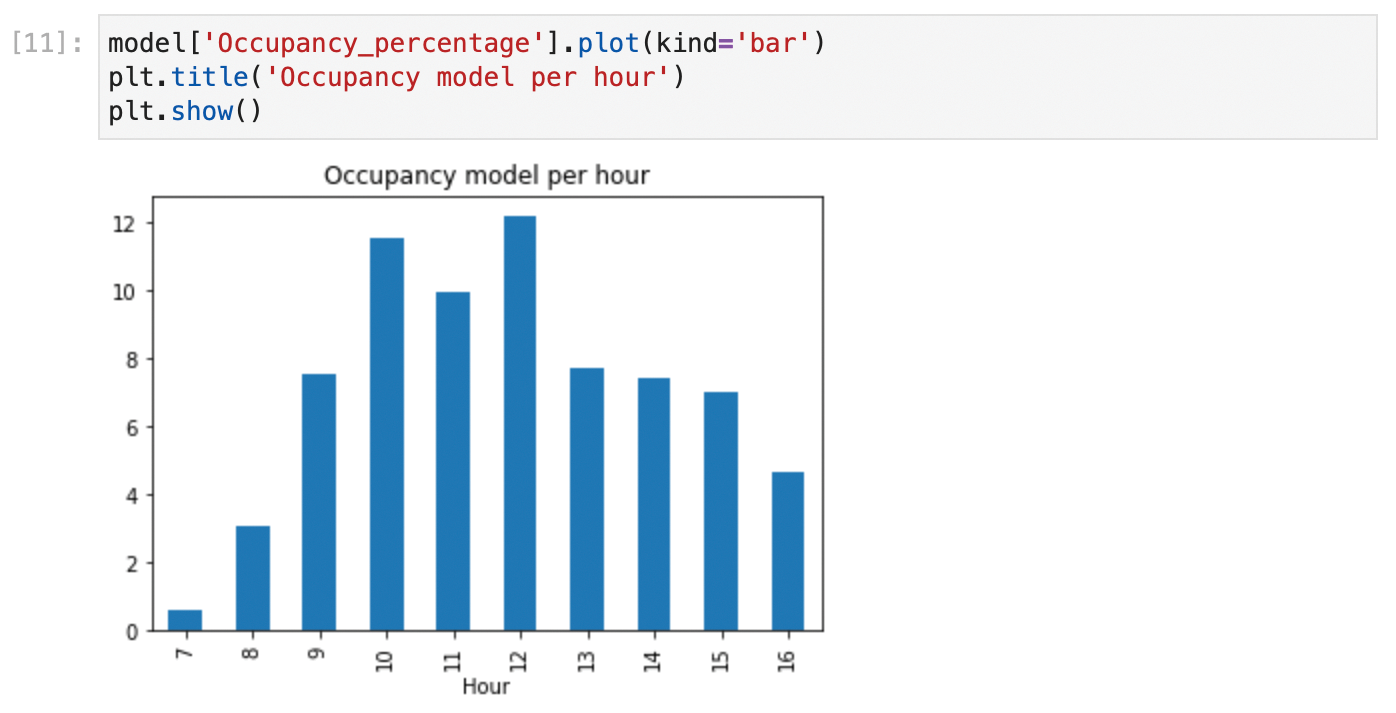
In this simple example, the data mining process was intentionally trivial. In some cases, the grouping and averaging operation can even be a part of the transformation step. Data mining can be very complex, including ML/AI processes, different kinds of numerical methods, and other advanced techniques. But there is one secret that all data analysts learn sooner or later: Most of the hard work of the data analytics process is already done before the data mining step. You can now use the model to represent a chart with the occupancy of the parking lot as a percentage for different hours of the day (Figure 14). More complex projects might involve live charts or detailed reports that are sent automatically by email to interested parties.
Conclusions
This article has been a primer on data science. I described how to take the KDD model as the outline for a typical workflow in a data analytics project. You also learned about the main Python libraries used with data science projects. Finally, I reviewed how to get the environment up and running, and I presented a simple example showing how to use it. This brief introduction is just the beginning. I'll leave it to you to discover how to apply the rich Python data analytics ecosystem to the problems you encounter in your own field of expertise.
Info
- Fayyad, U., G. Piatetsky-Shapiro, and P. Smyth, "The KDD process for extracting useful knowledge from volumes of data," Communications of the ACM, 39(11), 1996, pp. 27-34
- Stolfi, Daniel H., Enrique Alba, and Xin Yao. "Predicting Car Park Occupancy Rates in Smart Cities." In: Smart Cities: Second International Conference, Smart-CT 2017, M·laga, Spain, June 14-16, 2017, pp. 107-117
This article originally appeared in Linux Magazine and is reprinted here with permission.
Want to read more? Check out the latest edition of Linux Magazine.


Comments