
If you want to embed documentation in your code that goes beyond simple code comments or if you plan to give a presentation that includes some live hacking, try JupyterLab and create “notebooks” that can display and execute your code. As the Jupyter team explain in their documentation, “a notebook is a shareable document that combines computer code, plain language descriptions, data, rich visualizations like 3D models, charts, graphs and figures, and interactive controls.”
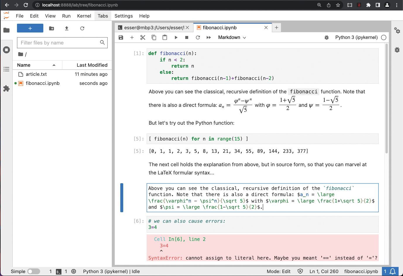
Working with a Jupyter notebook is similar to using an interpreter interactively: You can type in commands and have them executed directly. But in the notebook, every command, variable declation, or function implementation lives in what is called a cell. Those cells are code cells by default, but you can also use comment cells that accept documentation in Markdown syntax. Depending on which add-ons you add, you can embed LaTeX code in the markdown and have formulas displayed properly (Figure 1).
JupyterLab is a web-based Python program, and it supports several (interpreted) languages, including – of course – Python; the full list of languages is available online. When you launch a JupyterLab session you’ll get a new browser tab from which you can use the software.
In a JupyterLab session you can create one or more notebooks, and each notebook can use a different “kernel.” The kernel decides on the programming language that you can use in the code cells. You’ll get syntax highlighting, and when you press Shift+Return, the cell content is run through an interpreter. Cells are not isolated from one another. You are using one interpreter that will execute any code you send to it, so variables will keep their values and functions remain defined. Of course, there’s a reset option that lets you start with a fresh interpreter.
You can save the notebooks you create as *.ipynb files and pass them around, or put them online, for example, on GitHub or GitLab. A notebook file contains both all the cells (code and documentation) and any output that you’ve generated by running some of the cells. You don’t have to run all the cells, so you can send a notebook to a colleague or a student (if you’re teaching) and ask them to run the cells themselves to discover what the code does.
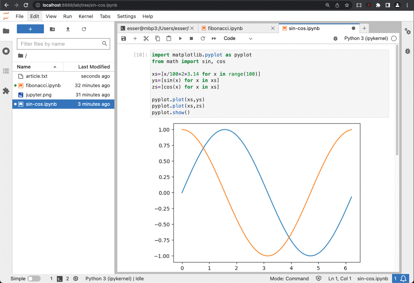
Creating graphics is easy, too: In Python, just import the matplotlib.pyplot module and use the plot function to draw dots. There are various ways to visualize data. Where a normal Python session would open a fresh window to display the graphics, JupyterLab embeds it in the notebook (Figure 2).
For installing JupyterLab, use Python’s own package manager pip and sudo pip install jupyterlab. On openSUSE you can also use Zypper (zypper in jupyter‑jupyterlab).
This article originally appeared in Cool Linux Hacks and is reprinted here with permission.
Want to read more? Check out the latest edition of Cool Linux Hacks.


Comments